When I first started trying wrap my mind around the concept of quadrature signals, I struggled to visualize what the signals represented in the physical world. It just didn’t seem intuitive. However, if memory serves me correctly, there was an old Java-based web site maintained by an engineer that contained interactive widgets to visualize the signals. I emailed the curator but received no response and the site eventually disappeared, so I promised myself to eventually recreate it. Hopefully, you will find this post helpful in strengthening your understanding of quadrature singals and digital communications. The interactive widgets are React JS components and will hopefully help you visualize the mathematics behind the concepts.

In Part 1 of our wireless transmission series, we looked at how binary data can be transmitted by switching an RF carrier on and off—On-Off Keying (OOK)—and why smoothing those amplitude transitions is critical for controlling spectral sidelobes.

While simple amplitude switching is easy to build, varying the amplitude of a carrier wave alone has two fundamental drawbacks in wireless links:

1. Limited Signal-Space Utilization: Encoding information only in carrier amplitude uses a single dimension of the available two-dimensional I/Q signal space, limiting how efficiently distinct symbols can be separated for a given average signal power.
2. Power-Efficiency Tradeoffs: Packing more amplitude levels onto a single dimension reduces the distance between adjacent symbols for a given average power, making reliable detection increasingly demanding as the constellation grows.

To pack more bits per second into a narrow channel, modern communications and radar systems encode information into both the phase and amplitude of the carrier wave using In-Phase ($I$) and Quadrature ($Q$) modulation.

How This Article Is Organized

To make this guide useful whether you are encountering I/Q data for the very first time or designing a physical FPGA/SDR transceiver, the article is structured in two progressive layers:

• Part I — Core Digital Modulation (Sections 1–4): Builds the complete conceptual foundation from first principles: Carrier $\rightarrow$ I/Q & Complex Baseband ($I + jQ$) $\rightarrow$ Bits, Symbols & Baud Rate $\rightarrow$ BPSK, QPSK & QAM $\rightarrow$ Noise, Decision Boundaries & Gray Coding.
• Part II — Making a Real Radio Work (Sections 5–7): Explores the practical RF hardware and DSP engineering required to transmit and recover those symbols over the air: PA Linearity & OQPSK $\rightarrow$ Nyquist Pulse Shaping (RRC) & Matched Filtering $\rightarrow$ Coherent Downconversion & Live Costas Loop Carrier Recovery.

At every step, keep this single End-to-End Digital Radio Signal Chain in mind—every concept and interactive lab in this article fits directly into one of these blocks:

flowchart LR
T1(["Input Bits<br/>0 1 1 0..."]) --> T2["Symbol Mapper<br/>(Gray Code)"] --> T3["Complex Baseband<br/>z = I + jQ"] --> T4["Pulse Shaping<br/>(TX RRC Filter)"] --> T5["I/Q Modulator<br/>s(t) = I·cos − Q·sin"]
classDef txNode fill:#1e1b4b,stroke:#6366f1,stroke-width:2px,color:#e0e7ff;
classDef ioNode fill:#0f172a,stroke:#38bdf8,stroke-width:2px,color:#e0f2fe;
class T2,T3,T4,T5 txNode;
class T1 ioNode;

flowchart LR
R1["I/Q Demodulator<br/>(Quadrature LO)"] --> R2["Matched Filter<br/>(RX RRC Filter)"] --> R3["Costas Loop PLL<br/>(Phase Derotation)"] --> R4["Decision Slicer<br/>(Nearest Symbol)"] --> R5(["Recovered<br/>Bits"])
classDef rxNode fill:#064e3b,stroke:#10b981,stroke-width:2px,color:#d1fae5;
classDef ioNode fill:#0f172a,stroke:#38bdf8,stroke-width:2px,color:#e0f2fe;
class R1,R2,R3,R4 rxNode;
class R5 ioNode;

Part I: Core Digital Modulation (From Carrier Wave to Constellations & Decisions)

1. What Can We Change About a Carrier, What Are I/Q, and What Is Complex Baseband?

1.1 The Three Knobs of a Sine Wave

At the heart of every wireless transmitter is a pure sinusoidal RF carrier wave:

If we want to embed information onto that wave, nature gives us only three physical parameters (“knobs”) we can vary over time:

1. Amplitude ($A$): The peak height (envelope) of the wave.
2. Frequency ($f_c$): How rapidly the wave oscillates per second.
3. Phase ($\phi$): The starting angular offset of the wave relative to a time-zero reference clock (measured in degrees from $-180^\circ$ to $+180^\circ$, or radians from $-\pi$ to $+\pi$).

Digital modulation works by deliberately stepping one or more of these parameters between a finite set of discrete, pre-agreed states. Before looking at how hardware controls phase, use the interactive explorer below to adjust Amplitude ($A$), Frequency ($f$), and Phase ($\phi$) against a fixed reference carrier:

1.2 Why Hardware Radios Don’t Shift Phase Directly: The Two-Dial I/Q Solution

Suppose we want to transmit data by shifting the phase $\phi(t)$ of a $2.4\text{ GHz}$ carrier wave to any arbitrary angle—say, $45^\circ$, $135^\circ$, or $-60^\circ$.

Directly building an electronically variable delay line or shifting the phase of a multi-gigahertz crystal oscillator linearly and instantaneously across $360^\circ$ without corrupting its frequency stability is a hardware nightmare.

Fortunately, a fundamental trigonometric angle-sum identity rescues us:

Look closely at what this equation reveals:

• Instead of trying to reach inside a high-frequency oscillator to twist its phase angle $\phi$ directly, we only need two fixed, $90^\circ$-shifted carrier waves from the same local oscillator: a $\cos(\omega_c t)$ wave (In-Phase) and a $\sin(\omega_c t)$ wave (Quadrature, shifted by a quarter-cycle, $90^\circ$).
• We multiply those two fixed waves by two simple baseband DC/low-frequency voltages—$I$ and $Q$—and add them together:

where the polar-to-Cartesian conversion is simply:

and the inverse Cartesian-to-polar relationship is:

The “Two Dials” Mental Model: Think of $I$ and $Q$ as an Etch-a-Sketch for radio waves. Instead of turning a polar steering wheel ($\phi$) and throttle ($A$), you have two simple linear volume dials—one controlling the height of $\cos(\omega_c t)$ ($I$) and one controlling the height of $-\sin(\omega_c t)$ ($Q$). By setting just those two voltages $(I, Q)$, their sum automatically synthesizes any amplitude $A$ and any phase angle $\phi$ across all $360^\circ$!

1.3 Complex Baseband ($z(t) = I(t) + jQ(t)$): One Complex Number Equals Amplitude & Phase

In digital signal processing (DSP) and software-defined radio (SDR), we package the two real baseband signals $I(t)$ and $Q(t)$ into a single Complex Baseband Signal $z(t)$ using Euler’s formula ($e^{j\phi} = \cos\phi + j\sin\phi$, where $j = \sqrt{-1}$):

Therefore, the instantaneous RF envelope amplitude $A(t)$ and phase $\phi(t)$ are simply the magnitude and angle of the complex number $z(t)$:

Key Takeaway: A digital radio can represent the instantaneous amplitude and phase of a modulated signal with a single complex number.

When you write a single line of Python or MATLAB code in an SDR flowgraph:

# Complex baseband I/Q sample stream in NumPy / GNU Radio / USRP / bladeRF
z = I + 1j*Q
amplitude = np.abs(z)      # Instantaneous RF envelope A(t)
phase_rad = np.angle(z)    # Instantaneous RF phase angle phi(t)

this is far more than convenient software shorthand—z = I + 1j*Q is the exact mathematical representation of the physical signal prior to upconversion. Every SDR hardware interface (USRP, bladeRF, PlutoSDR, RTL-SDR), FFT spectrum analyzer, and digital baseband equalizer operates directly on arrays of these complex numbers $z[n] = I[n] + jQ[n]$.

1.4 Why Do We Call Them “Orthogonal”?

Why do we pick $\cos(\omega_c t)$ and $\sin(\omega_c t)$—waves separated by $90^\circ$—rather than two waves separated by $30^\circ$ or $60^\circ$?

The cosine and sine basis functions form orthogonal quadrature components under coherent detection. This allows the receiver to independently recover the $I$ and $Q$ projections of the transmitted signal.

This zero cross-term holds over an integer number of carrier cycles (or an equivalent coherent observation interval), which is why an ideal coherent receiver can project the received waveform independently onto the $I$ and $Q$ basis functions.

When a coherent receiver multiplies the incoming passband waveform $s(t) = I(t)\cos(\omega_c t) - Q(t)\sin(\omega_c t)$ by synchronized local $\cos(\omega_c t)$ and $-\sin(\omega_c t)$ oscillators and low-pass filters the resulting double-frequency ($2f_c$) mixer terms (assuming $f_c \gg R_s$), the ideal cross-term between the two rails vanishes after coherent demodulation and low-pass filtering. Under ideal coherent synchronization, this allows the $I$ and $Q$ projections to be recovered as independent orthogonal components on the same RF carrier frequency at the same time—a result we derive step-by-step in Section 7.

1.5 Interactive Lab: The I/Q Phasor & Waveform Synthesizer

Drag the In-Phase ($I$) and Quadrature ($Q$) sliders (or click the quick phase presets) below to see how setting two DC levels $(I, Q)$ moves the complex phasor $z = I + jQ$ on the constellation plane and synthesizes the exact passband RF wave $s(t)$:

2. Bits, Symbols, and Baud Rate ($R_b = R_s \log_2 M$)

Before introducing specific digital modulation formats like BPSK, QPSK, or QAM, we need the single most important bridge between digital software and analog radio waves: the difference between a Bit and a Symbol.

In digital communications, a transmitter does not necessarily send raw bits (0 and 1) one at a time. Instead, the Symbol Mapper groups the incoming binary stream into chunks of $k$ bits and selects one Symbol from an alphabet of $M = 2^k$ allowed $(I, Q)$ coordinates:

Compare how BPSK ($1\text{ bit per symbol}$) and QPSK ($2\text{ bits per symbol}$) process the exact same 8-bit sequence 0 1 1 0 1 0 0 1:

1. BPSK (M = 2 allowed states → k = 1 bit per symbol):
   Input Bits:      0   |   1   |   1   |   0   |   1   |   0   |   0   |   1
                    ↓       ↓       ↓       ↓       ↓       ↓       ↓       ↓
   Symbols Sent:   S0      S1      S1      S0      S1      S0      S0      S1   (8 symbols required)

2. QPSK (M = 4 allowed states → k = 2 bits per symbol):
   Input Bit Pairs:   01    |     10    |     10    |     01
                      ↓           ↓           ↓           ↓
   Symbols Sent:      S1          S2          S2          S1                    (Only 4 symbols required!)

Symbol Rate (Baud, $R_s$) vs. Bit Rate ($R_b$)

• Symbol Rate ($R_s = 1 / T_s$, measured in $\text{symbols/sec}$ or $\text{Baud}$): How many times per second the radio changes from one modulation symbol to the next.
• Bit Rate ($R_b$, measured in $\text{bits/sec}$): The raw bit rate represented by the modulation, related to the symbol rate $R_s$ and constellation size $M$ by:

Symbol rate sets the fundamental time scale of the waveform, but the actual occupied bandwidth also depends on the pulse-shaping filter; for example, a Raised-Cosine response with roll-off $\alpha$ has one-sided baseband bandwidth $(1+\alpha)R_s/2$.

Bandwidth vs. Modulation Order: For a fixed pulse-shaping filter and roll-off factor $\alpha$, nominal null-to-null RF bandwidth is primarily determined by symbol rate $R_s$ ($B_{\text{RF}} = (1 + \alpha)R_s$), rather than the number of bits represented by each symbol. Increasing $M$ therefore increases the bit rate $R_b$ at a fixed symbol rate without increasing the nominal occupied bandwidth, assuming the same pulse shaping.

This relationship explains the motivation for the modern digital modulation ladder:

Let’s walk up this modulation ladder step by step.

3. Walking Up the Modulation Ladder: BPSK ($M=2$), QPSK ($M=4$), and QAM ($M=16, 64, 256$)

3.1 Binary Phase Shift Keying (BPSK): $M = 2 \implies 1\text{ bit/symbol}$

The simplest phase modulation format uses only $M = 2$ symbols separated by $180^\circ$ along the In-Phase ($I$) axis while keeping the Quadrature ($Q$) rail permanently set to zero:

• Bit 0 ($S_0$): $I = +1, Q = 0 \implies s(t) = +\cos(\omega_c t)$ ($\phi = 0^\circ$)
• Bit 1 ($S_1$): $I = -1, Q = 0 \implies s(t) = -\cos(\omega_c t) = \cos(\omega_c t + 180^\circ)$ ($\phi = 180^\circ$)

Because BPSK places both points on the horizontal $I$ axis ($Q = 0$), it leaves the entire vertical Quadrature ($Q$) dimension unused.

3.2 Quadrature Phase Shift Keying (QPSK): $M = 4 \implies 2\text{ bits/symbol}$

Each QPSK symbol contains two bits. In the rectangular mapping used here, one bit determines the sign of $I$ and the other determines the sign of $Q$, selecting one of $M = 4$ allowed $(I + jQ)$ coordinates equally spaced around the unit circle ($A = \sqrt{I^2 + Q^2} = 1$):

Because each QPSK symbol represents 2 bits instead of 1, QPSK doubles the bit rate at a fixed symbol rate $R_s$ (or, for the same pulse-shaping roll-off, halves the symbol rate and nominal occupied bandwidth needed to carry a given raw bit rate $R_b$)!

Interactive Comparator: BPSK ($M=2$) vs. QPSK ($M=4$)

Click any of the 8 input bits (0 or 1) below to compare how BPSK sends 8 individual 1-bit symbols while QPSK groups them into 4 two-bit symbols ($T_s = 2T_b$):

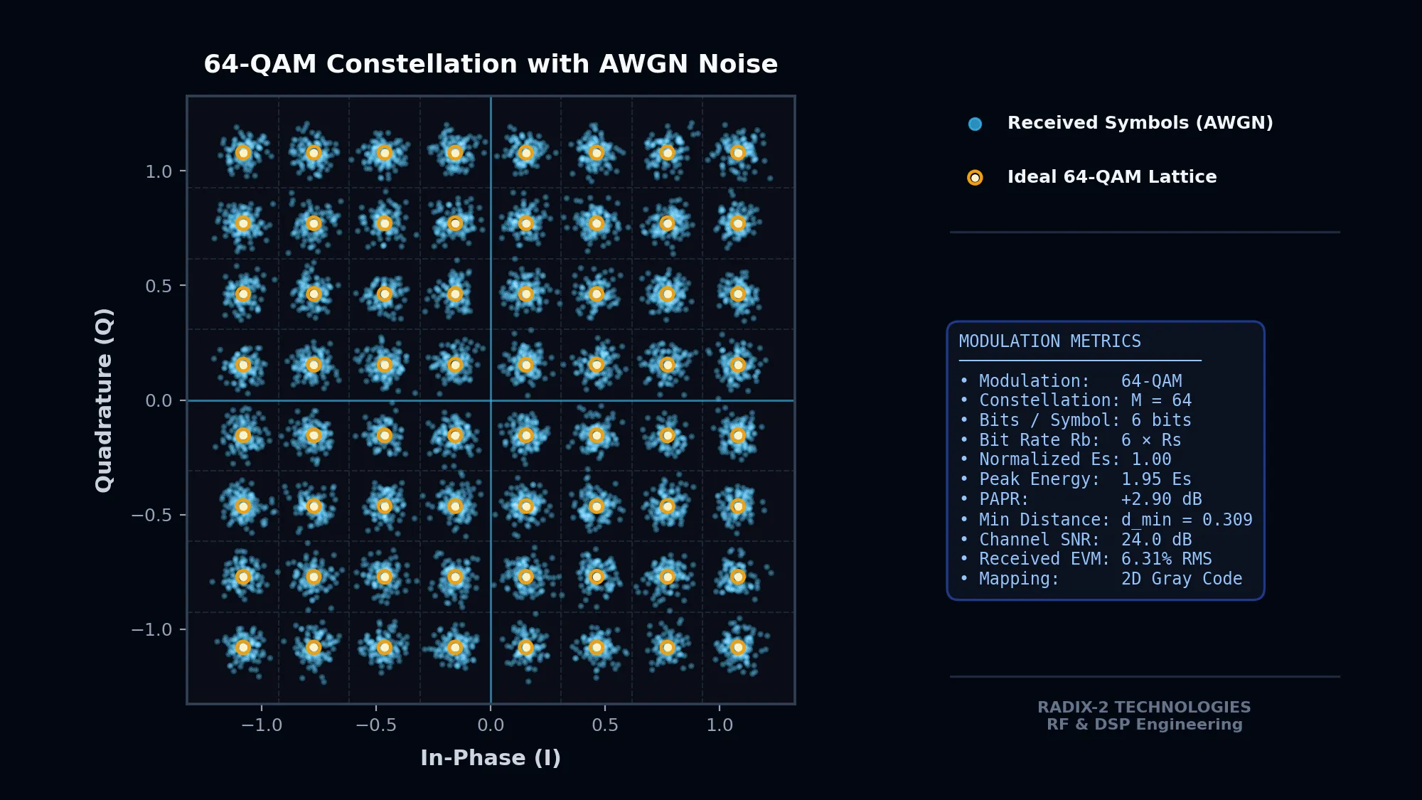
3.3 Extending the Exact Same Grid: Quadrature Amplitude Modulation (16-QAM, 64-QAM, and 256-QAM)

Once you understand QPSK as selecting from $2$ voltage levels on $I$ ($\pm 1$) and $2$ voltage levels on $Q$ ($\pm 1$) to form a $2 \times 2 = 4$-point grid, Quadrature Amplitude Modulation ($M\text{-QAM}$) is simply the natural continuation of the exact same idea!

Instead of restricting our $I$ and $Q$ Digital-to-Analog Converters (DACs) to only 2 binary levels ($\pm 1$), we allow $I$ and $Q$ to step across $L = \sqrt{M}$ evenly spaced discrete amplitude levels on each of the $I$ and $Q$ axes:

• 16-QAM ($M = 16 \implies 4\text{ bits/symbol}$): The first $2$ bits choose from $4$ levels on $I$ ($\{-3, -1, +1, +3\}$) and the next $2$ bits choose from $4$ levels on $Q$ ($\{-3, -1, +1, +3\}$), forming a $4 \times 4 = 16$-point grid.
• 64-QAM ($M = 64 \implies 6\text{ bits/symbol}$): $3$ bits on $I$ ($8$ levels) $\times$ $3$ bits on $Q$ ($8$ levels) = $8 \times 8 = 64$-point grid.
• 256-QAM ($M = 256 \implies 8\text{ bits/symbol}$): $4$ bits on $I$ ($16$ levels) $\times$ $4$ bits on $Q$ ($16$ levels) = $16 \times 16 = 256$-point grid.

Why arrange the points in a 2D square grid instead of placing 16 or 64 phase angles around a single circle ($16\text{-PSK}$ or $64\text{-PSK}$)? Because crowding 16 or 64 symbols onto the perimeter of a 1D circle wastes the entire interior of the $I/Q$ plane! Spreading the points across a 2D square grid modulates both amplitude $A(t)$ and phase $\phi(t)$, keeping neighboring points much farther apart (about a $4.2\text{ dB}$ advantage in normalized squared minimum Euclidean distance for 16-QAM versus 16-PSK at equal average symbol energy).

Interactive Explorer: 16-QAM vs. 64-QAM vs. 256-QAM

Switch between 16-QAM, 64-QAM, and 256-QAM below. Click any symbol slot (S1–S4) and click any point on the constellation grid to see how its $(I, Q)$ coordinates control the amplitude and phase of the RF waveform:

4. Noise, Decision Boundaries, Euclidean Distance ($d_{\min}$), and Gray Coding

If 256-QAM transmits $8\text{ bits/symbol}$—eight times the raw bit rate of BPSK at the same symbol rate and nominal pulse-shaped bandwidth—why don’t we use 256-QAM or 4096-QAM on every deep-space probe and weak-signal link?

The answer lies in what happens inside the RF Channel and the Receiver Symbol Slicer.

4.1 Additive White Gaussian Noise (AWGN): Why Received Points Form a Cloud

When a radio wave travels through space and enters a receiver front-end amplifier, random noise from the propagation channel and receiver—often modeled as thermal-noise-dominated—adds an unpredictable complex noise sample $n[k] = n_I[k] + j n_Q[k]$. In the standard Additive White Gaussian Noise (AWGN) model:

In the standard complex-baseband AWGN model, $n_I$ and $n_Q$ are independent zero-mean Gaussian components with equal variance. The exact relationship between that variance and $N_0$ depends on the one-sided/two-sided PSD convention, so this article uses $E_b/N_0$ and $E_s/N_0$ without requiring a particular discrete-time noise-variance normalization.

After receive filtering and sampling, the resulting Gaussian noise perturbation causes constellation samples to form a fuzzy 2D Gaussian cloud centered around each ideal transmitted coordinate:

   Transmitted Symbol (TX)             Received Symbol Cloud (RX + Noise)
                                                    .  .
              •                                  .   •   .
                                                   .   .

The spread of this noise cloud relative to the signal power is quantified by two closely related metrics:

• Energy-to-Noise-Density Ratios ($E_s / N_0$ and $E_b / N_0$): The symbol-energy-to-noise-density ratio $E_s/N_0$ and bit-energy-to-noise-density ratio $E_b/N_0$ normalize signal energy to the noise power spectral-density parameter $N_0$. For an uncoded $M$-ary modulation carrying $k=\log_2M$ bits per symbol, $E_s=kE_b=E_b\log_2M$. These quantities are closely related to SNR but allow modulation schemes with different symbol and bit rates to be compared on a common energy basis.
• Error Vector Magnitude ($\text{EVM}_{\text{rms}}$): The root-mean-square length of the error vector $\vec{e}[k] = z_{\text{RX}}[k] - z_{\text{TX}}[k]$ expressed as a percentage of the constellation reference amplitude. For a correctly normalized signal impaired only by uncorrelated AWGN, and with signal and noise powers evaluated over the same measurement bandwidth, $\text{EVM}_{\text{rms}} \approx 10^{-\text{SNR}_{\text{dB}}/20} \times 100\%$. (In a physical radio transceiver, measured EVM also includes contributions from carrier phase noise, residual frequency offset, I/Q gain and quadrature imbalance, non-linear PA distortion, timing error, and DAC/ADC quantization.)

4.2 Receiver Decision Boundaries & Minimum Euclidean Distance ($d_{\min}$)

The receiver does not know which symbol was transmitted; it only sees the noisy coordinate $z_{\text{RX}} = (I_{\text{RX}}, Q_{\text{RX}})$. For equally likely symbols in AWGN, Maximum Likelihood detection reduces to minimum-Euclidean-distance detection: the receiver partitions the $I/Q$ plane with Decision Boundaries (the perpendicular bisectors halfway between neighboring constellation points) and picks whichever valid symbol lies closest to $z_{\text{RX}}$.

A Symbol Error occurs whenever a random noise gust pushes $z_{\text{RX}}$ by more than half the distance to the nearest neighbor ($d_{\min} / 2$), crossing a decision boundary!

For a fixed average transmit power ($E_s = 1$), packing more points into the $I/Q$ plane shrinks the Minimum Euclidean Distance ($d_{\min}$) between neighboring symbols:

Because each modulation carries a different number of bits per symbol, $E_s/N_0$ should not be interpreted directly as energy efficiency per information bit; for uncoded modulation, the corresponding value is $E_b/N_0=(E_s/N_0)/\log_2M$ in linear units, or $(E_b/N_0)_{\text{dB}}=(E_s/N_0)_{\text{dB}}-10\log_{10}(\log_2M)$.

4.3 Why Gray Coding (00 $\rightarrow$ 01 $\rightarrow$ 11 $\rightarrow$ 10) Minimizes Bit Errors from Nearest-Neighbor Symbol Errors

Once we understand decision boundaries, the reason for Gray Coding becomes immediately obvious.

When noise causes a symbol error at normal operating SNR, the received dot almost always spills across a single boundary into an immediately adjacent cell (distance $d_{\min}$) rather than jumping all the way across the constellation.

• If we labeled our four QPSK quadrants in Natural Binary counting order (00 $\rightarrow$ 01 $\rightarrow$ 10 $\rightarrow$ 11), crossing the single boundary between 01 ($135^\circ$) and 10 ($225^\circ$) would flip both bits at once ($2\text{ bit errors}$ from $1\text{ symbol error}$)!
• By labeling adjacent cells using Gray Code (00 $\rightarrow$ 10 $\rightarrow$ 11 $\rightarrow$ 01), every pair of neighboring symbols sharing a decision boundary differs by exactly 1 bit. Thus, a nearest-neighbor symbol error corrupts only $1$ bit out of $\log_2(M)$, minimizing the Bit Error Rate (BER)!

Interactive Lab: Noise Cloud, Decision Boundaries & Gray Coding vs. Natural Binary

Use the interactive explorer below to adjust the Channel SNR ($E_s/N_0$) across BPSK, QPSK, and 16-QAM, see the red dashed Decision Boundaries, and toggle between Gray Coding and Natural Binary to see how Gray coding reduces the Bit Error Rate:

Timing-Recovery Assumption: To keep this article focused on carrier phase recovery, we assume the receiver has already acquired symbol timing and knows the correct matched-filter sampling instants. Practical receivers recover this timing separately using timing-error detectors such as Gardner or Mueller-and-Müller with an interpolator/NCO loop; that topic will be covered in a later receiver-synchronization article.

Part II: Making a Real Radio Work — Practical RF & DSP Implementation

5. Spectral Occupied Bandwidth, Nyquist Baseband Pulse Shaping (RC / RRC), & Matched Filtering

(Signal-Chain Blocks: Transmit Pulse Shaping & Receiver Matched Filter)

In Sections 2 and 3, we sketched our baseband $I(t)$ and $Q(t)$ signals as sharp rectangular voltage steps of duration $T_s$. Why can’t we send raw rectangular steps directly to the antenna?

5.1 Why Rectangular Steps Spill Across the RF Spectrum

By the Fourier Transform, a sharp rectangular pulse $\text{rect}(t / T_s)$ of duration $T_s = 1 / R_s$ in the time domain transforms into a wide $\text{sinc}(f T_s)$ spectrum in the frequency domain. Upconverted to $f_c$, its Power Spectral Density (PSD) is:

The first spectral sidelobe of $\text{sinc}^2(f T_s)$ sits only $-13.3\text{ dB}$ below the main carrier lobe, and subsequent sidelobes decay slowly at $1/f^2$ ($-6\text{ dB/octave}$), spraying wideband interference across neighboring radio channels.

5.2 Nyquist’s First Criterion: Band-Limiting Without Inter-Symbol Interference (ISI)

To confine the transmitted signal to a tight RF channel bandwidth $B_{\text{RF}}$, we must pass our discrete complex symbols $z[k] = I[k] + jQ[k]$ through a band-limiting low-pass pulse-shaping filter $p(t)$.

Low-pass filtering stretches each symbol into a smooth oscillating wave spanning several symbol periods ($-3T_s \dots +3T_s$). How do we keep the ringing tails of preceding symbols from corrupting the current symbol (Inter-Symbol Interference, ISI)?

For a synchronized linear pulse-amplitude modulation system, zero ISI at the symbol decision instants ($t = kT_s$) is obtained when the end-to-end pulse $p(t)$ satisfies the time-domain form of Nyquist’s First Criterion:

In other words, the pulse can oscillate between samples as long as its zero-crossings land at every integer multiple of the symbol period ($\pm T_s, \pm 2T_s, \pm 3T_s, \dots$)! At the exact instant the receiver samples symbol $k$, the tails of all other symbols pass through $0.00\text{ V}$.

5.3 The Raised-Cosine (RC) & Root-Raised-Cosine (RRC) Matched Filter Pair

Practical digital radios use the Raised-Cosine (RC) pulse family, parameterized by the Roll-Off Factor $\alpha \in [0, 1]$ (excess bandwidth factor):

which bounds the total occupied RF passband bandwidth to:

The PAPR values below are representative results for a particular pulse-shaped QPSK sequence and filter implementation; unlike occupied bandwidth, waveform PAPR is not determined by $\alpha$ alone.

Interactive Lab: Nyquist Pulse Shaping, Spectrum & Zero-ISI Superposition

Use the interactive lab below to switch between Unfiltered Rect, TX Only (Single RRC), and TX + RX Cascade (Raised-Cosine), drag the Roll-Off Factor ($\alpha$) slider, and observe how all 6 overlapping symbol pulses sum to zero ISI at the symbol decision instants marked by the green sampling strobes ($t = kT_s$):

6. RF Transmitter Limitations: $180^\circ$ Envelope Collapse, PA Compression, and Why OQPSK Exists

(Signal-Chain Block: I/Q Modulator & RF Power Amplifier)

Now that we see how Root-Raised-Cosine filtering smooths $I(t)$ and $Q(t)$ between symbols, we can understand a critical RF hardware trap. On paper, QPSK looks like a constant-envelope modulation because all four constellation points lie on the unit circle ($A = \sqrt{I^2 + Q^2} = 1$). Once pulse-shaped, however, QPSK is NOT constant-envelope.

6.1 Idealized $180^\circ$ Origin Crossings & Pulse-Shaped Envelope Excursions

With idealized simultaneous $I/Q$ transitions, a $180^\circ$ QPSK transition (such as 00 at $45^\circ \to$ 11 at $225^\circ$, or 10 at $135^\circ \to$ 01 at $315^\circ$) passes directly through the origin $(I=0, Q=0)$, producing a momentary $100\%$ envelope null. Multi-symbol RRC pulse shaping modifies the exact inter-symbol trajectory depending on the filter roll-off $\alpha$ and surrounding symbols, but $180^\circ$ phase reversals still cause deep envelope dips and large peak-to-average envelope excursions.

When a pulse-shaped waveform with deep envelope dips and $+3\text{ dB}$ overshoots drives a high-efficiency RF Power Amplifier (PA) operating near compression ($P_{1\text{dB}}$), the amplifier’s non-linear AM-to-AM (gain compression) and AM-to-PM (phase rotation vs. drive level) distortion violently regenerates the outer spectral sidelobes (spectral regrowth)—undoing the spectral containment of our RRC filter!

6.2 The Hardware Solution: Offset-QPSK (OQPSK)

By inserting a half-symbol delay ($T_b = T_s / 2$) into the Quadrature ($Q$) baseband path before the mixer, $I(t)$ and $Q(t)$ never transition at the same instant:

• At even bit intervals ($t = 0, 2T_b, 4T_b\dots$), only $I(t)$ can transition while $Q(t)$ holds steady.
• At odd bit intervals ($t = T_b, 3T_b, 5T_b\dots$), only $Q(t)$ can transition while $I(t)$ holds steady.

Because only one coordinate can change sign at a time, $180^\circ$ diagonal transitions through the origin $(0,0)$ are eliminated. The phase never steps by more than $\pm 90^\circ$, so that in the idealized rectangular-pulse trajectory the envelope does not pass through zero; with practical pulse shaping, the exact minimum envelope depends on the filter and surrounding symbol sequence, substantially reducing envelope fluctuations and allowing satellite and tactical RF power amplifiers to operate efficiently near saturation. (Tip: Scroll back to the interactive Phase Modulation Comparator in Section 3 and toggle between QPSK and OQPSK to compare their constellation trajectories.)

7. Coherent Demodulation, Quadrature Downconversion, & Costas Loop Carrier Recovery

(Signal-Chain Blocks: I/Q Demodulator & Carrier Phase Recovery)

We now arrive at the final link in our signal chain: when only a single real passband voltage $s(t) = I(t)\cos(\omega_c t + \theta_{\text{TX}}) - Q(t)\sin(\omega_c t + \theta_{\text{TX}})$ reaches the receiver antenna, how does the receiver separate $I(t)$ and $Q(t)$ and lock onto the transmitter’s phase without a reference wire?

7.1 Consistent Phase-Error Sign Convention & Coherent Quadrature Downconversion

Let’s define our phase convention explicitly so that the mixer equations, baseband rotation matrix, constellation plot, and Costas loop equations are $100\%$ consistent:

• Let the incoming transmitted RF wave have instantaneous carrier phase $\Phi_{\text{TX}}(t) = \omega_c t + \theta_{\text{TX}}(t)$: $s(t) = I(t)\cos\big(\omega_c t + \theta_{\text{TX}}(t)\big) - Q(t)\sin\big(\omega_c t + \theta_{\text{TX}}(t)\big)$
• Let the receiver’s Local Oscillator (LO) have instantaneous phase $\Phi_{\text{LO}}(t) = \omega_c t + \theta_{\text{LO}}(t)$, driving two quadrature downconversion mixers:
  • Top ($I_{\text{RX}}$) Mixer: Multiplies $s(t)$ by $+2\cos\big(\omega_c t + \theta_{\text{LO}}(t)\big)$ followed by the RRC Low-Pass Matched Filter.
  • Bottom ($Q_{\text{RX}}$) Mixer: Multiplies $s(t)$ by $-2\sin\big(\omega_c t + \theta_{\text{LO}}(t)\big)$ followed by an identical Low-Pass Matched Filter.
• Define the Channel / Receiver Phase Error $\theta_e(t)$ as the phase of the incoming TX carrier relative to the receiver LO: $\theta_e(t) \;\triangleq\; \theta_{\text{TX}}(t) - \theta_{\text{LO}}(t) \;=\; (\omega_c - \omega_{\text{LO}})t + \theta_0 \;=\; 2\pi \Delta f\,t + \theta_0$

Applying the product-to-sum identities ($2\cos A \cos B = \cos(A - B) + \cos(A + B)$ and $2\sin A \cos B = \sin(A - B) + \sin(A + B)$) with $A = \omega_c t + \theta_{\text{TX}}$ and $B = \omega_c t + \theta_{\text{LO}}$ (so that the difference angle is $A - B = \theta_{\text{TX}} - \theta_{\text{LO}} = \theta_e$), the upper mixer output before low-pass filtering is:

And similarly for the lower mixer $s(t)\cdot\big(-2\sin(\omega_c t + \theta_{\text{LO}})\big)$, after the Low-Pass Matched Filter strips away the $2f_c$ terms, we obtain the exact downconverted baseband outputs:

Notice two critical results from this single derivation:

1. When the Receiver LO Is Phase-Locked ($\theta_e = 0^\circ \implies \cos 0^\circ = 1, \sin 0^\circ = 0$): $I_{\text{RX}}(t) = I(t), \qquad Q_{\text{RX}}(t) = Q(t)$ With the $2f_c$ mixer products rejected by the low-pass matched filter and $\theta_e=0$, the remaining $I/Q$ cross-coupling terms are zero.
2. When a Phase Error $\theta_e(t) = \theta_{\text{TX}} - \theta_{\text{LO}} \ne 0$ Exists: Packaging $(I_{\text{RX}}, Q_{\text{RX}})$ into complex baseband $z_{\text{RX}}(t) = I_{\text{RX}}(t) + jQ_{\text{RX}}(t)$ yields the Complex Baseband Rotation: $z_{\text{RX}}(t) = \big(I(t) + jQ(t)\big)\big(\cos\theta_e(t) + j\sin\theta_e(t)\big) = z_{\text{TX}}(t)\cdot e^{+j\theta_e(t)}$ Or in $2 \times 2$ rotation matrix form: $\begin{bmatrix} I_{\text{RX}}(t) \\ Q_{\text{RX}}(t) \end{bmatrix} = \begin{bmatrix} \cos\theta_e(t) & -\sin\theta_e(t) \\ \sin\theta_e(t) & \cos\theta_e(t) \end{bmatrix} \begin{bmatrix} I(t) \\ Q(t) \end{bmatrix}$ (Note on sign conventions: If one instead defines phase error as the LO phase advance $\theta'_e \triangleq \theta_{\text{LO}} - \theta_{\text{TX}} = -\theta_e$, then substituting $-\theta'_e$ flips the sign of $\sin\theta_e$, giving $I_{\text{RX}} = I\cos\theta'_e + Q\sin\theta'_e$, $Q_{\text{RX}} = -I\sin\theta'_e + Q\cos\theta'_e$, and $z_{\text{RX}} = z_{\text{TX}}e^{-j\theta'_e}$. Both describe the exact same physical phenomenon: a mismatch between TX and LO phases rotates the complex constellation!)

7.2 The Costas Loop & $90^\circ$ Rotational Phase Ambiguity

Because suppressed-carrier BPSK, QPSK, and QAM signals have symmetric constellations ($\pm V$), their average carrier power at $f_c$ cancels to zero—leaving no discrete carrier tone for an ordinary PLL to track.

Instead, coherent receivers use a Decision-Directed Costas Loop:

• Phase Error Detector (PED): Strips away the data modulation using hard constellation decisions. For BPSK, a conventional multiplier-type Costas detector can form $e_\phi[k] = I_{\text{RX}}[k]Q_{\text{RX}}[k]$, with an ideal detector characteristic proportional to $\sin(2\theta_e)$; near lock, $\sin(2\theta_e)\approx2\theta_e$. Its $180^\circ$ periodicity produces the expected BPSK phase ambiguity. For QPSK, $\hat{I} = \text{sgn}(I_{\text{RX}})$ and $\hat{Q} = \text{sgn}(Q_{\text{RX}})$ identify the nearest quadrant. For higher-order QAM, the receiver instead uses a full constellation slicer $\hat{z}[k] = \hat{I}[k] + j\hat{Q}[k] = \text{slice}\{z_{\text{RX}}[k]\}$ that selects the nearest valid amplitude and phase state. A decision-directed phase-error detector can then be written compactly as: $e_\phi[k] = \operatorname{Im}\!\left\{z_{\text{RX}}[k]\hat{z}^{*}[k]\right\}$ For QPSK, this is equivalent (up to sign convention) to $Q_{\text{RX}}[k]\hat{I}[k] - I_{\text{RX}}[k]\hat{Q}[k]$. Because the QPSK constellation has fourfold rotational symmetry, the detector characteristic repeats every $90^\circ$, producing four possible carrier-phase lock orientations. Square QAM constellations have the same fourfold rotational symmetry, so decision-directed carrier recovery can retain the same $90^\circ$ phase ambiguity until pilots, differential encoding, or higher-layer framing resolve the absolute orientation. The Costas loop therefore performs carrier synchronization modulo the constellation symmetry; a known pilot, preamble, differential encoding, or framing constraint is what resolves the remaining absolute phase orientation.
• PI Loop Filter & NCO: Feeds $e_\phi[k]$ through a 2nd-order Proportional-Integral filter to advance the Numerically Controlled Oscillator (NCO) phase $\theta_{\text{LO}}$ until $\theta_e = \theta_{\text{TX}} - \theta_{\text{LO}} \to 0$.
• The $90^\circ$ Phase Ambiguity Problem: Because $\sin(4\theta_e)$ repeats four times every $360^\circ$, the Costas loop has 4 stable lock points ($0^\circ, +90^\circ, \pm 180^\circ, -90^\circ$). If the loop settles into $+90^\circ$, the constellation stops spinning and locks sharply—but every Quadrant I "00" symbol is rotated into Quadrant II ("10")! Real-world receivers resolve this by correlating against known Pilot / Preamble symbols (or by using differential encoding, DQPSK).

Interactive Lab: Real-Time Streaming Costas Loop & 90° Phase Ambiguity Simulator

Watch the live ~24 symbol/sec streaming Costas Loop below:

1. Click Open-Loop (Watch LO Spin!) to see how a tiny frequency offset $\Delta f$ causes the constellation to orbit continuously around the unit circle.
2. Click Engage Costas Loop PLL to watch the NCO grab the spinning stream, track out $\Delta f$, and pull the red operating ball into a stable zero-crossing valley on the S-curve!
3. Click ⚡ Kick +68° Step (Force 90° False Lock!) to watch the loop settle into the $+90^\circ$ ambiguity valley (where green "00" symbols stream into Quadrant II), then click Resolve 90°/180° Ambiguity via Pilot ("00") to derotate the live stream back to Quadrant I:

Summary & What’s Next in the Series

We have traveled all the way from a raw sinusoidal carrier $s(t) = A\cos(2\pi f_c t + \phi)$ to a complete single-carrier digital transceiver:

flowchart LR
M1(["Bit Stream<br/>Rb = Rs·log₂M"]) --> M2["Constellation<br/>zₖ = Iₖ + jQₖ"] --> M3["TX RRC Filter<br/>B_NN = (1+α)Rs"] --> M4["OQPSK / PA<br/>Avoid 180° Zero"] --> M5["RF Upconverter<br/>Re{z(t)·eʲ²πfᶜt}"]
classDef txNode fill:#1e1b4b,stroke:#6366f1,stroke-width:2px,color:#e0e7ff;
classDef ioNode fill:#0f172a,stroke:#38bdf8,stroke-width:2px,color:#e0f2fe;
class M2,M3,M4,M5 txNode;
class M1 ioNode;

flowchart LR
D1["I/Q Downconverter<br/>z_RX = z_TX·e⁺ʲθe"] --> D2["RX RRC Matched<br/>H_RRC² = H_RC (0 ISI at Sampling Instants)"] --> D3["Carrier Recovery<br/>Costas / Pilot-Aided<br/>z_corr = z_RX·e⁻ʲθ̂"] --> D4["Minimum-Distance Slicer<br/>arg min |z − z_m|²"] --> D5(["Decoded Bits<br/>Gray Mapped"])
classDef rxNode fill:#064e3b,stroke:#10b981,stroke-width:2px,color:#d1fae5;
classDef ioNode fill:#0f172a,stroke:#38bdf8,stroke-width:2px,color:#e0f2fe;
class D1,D2,D3,D4 rxNode;
class D5 ioNode;

1. Complex Baseband ($z = I + jQ$): Lets digital hardware steer any RF amplitude $A = |z|$ and phase $\phi = \angle z$ using simple Cartesian addition on two orthogonal $\cos(\omega_c t)$ and $-\sin(\omega_c t)$ carriers.
2. Modulation Order ($R_b = R_s \log_2 M$): Stepping from BPSK ($1\text{ bit/symbol}$) to QPSK ($2\text{ bits/symbol}$) to 16/64/256-QAM ($4\text{–}8\text{ bits/symbol}$) increases the raw modulation bit rate inside the same nominal symbol rate and nominal null-to-null RF bandwidth $B_{\text{RF}} = (1 + \alpha)R_s$, trading smaller symbol separation ($d_{\min}$) for higher spectral efficiency.
3. Practical Transceiver Engineering: Gray coding minimizes bit errors across decision boundaries; Root-Raised-Cosine (RRC) pulse shaping confines the transmitted spectrum, while the matched TX/RX RRC pair produces a Raised-Cosine response satisfying the zero-ISI criterion at the symbol decision instants; Offset-QPSK (OQPSK) prevents $180^\circ$ origin crossings; and Costas Loops + Pilot Preambles recover the suppressed carrier phase at the receiver.